GRAND VALLEY
STATE UNIVERSITY
MTH 380, Wavelets
Professor Edward Aboufadel
A Wavelets Approach to
Voice Recognition
by
Paul Hoekstra
November 29, 2001
1.0 Introduction:
Speech recognition has been an important part of the civilization for many centuries. We depend on intelligent and recognizable sounds for common communications. If each syllable is not enunciated in just the right fashion we are rendered incapable of vocally conveying our ideas, thoughts, and emotions.
Throughout history, mankind has utilized the human ear as our main receptor and analyzer for sounds. Our ears gather audible information and pass it on to the brain for processing. One piece of data that the ear gathers is the amplitude of the sound. It differentiates amplitude by the level of excitation that the follicles in the cochlea experience. The second piece of data that the ear gathers is pitch. Pitch is the measure of frequency, and is determined in the ear as the number of changes in pressure that occur in a given period of time. The third, and perhaps least intuitive, piece of information that the ear collects is the time that each amplitude and frequency occurs. Since we have a general perception of the passing of time, and we are provided with amplitudes and frequencies, we then know the time of occurrence for each amplitude and frequency pair.
Because the human brain is so adept at acquiring and recognizing sounds, it is natural to imitate the modus operandi of the human perception of sound. Since the data that is collected and processed by the brain consists of three variables, we should use all three of these variables in our analysis of sound. The collection of amplitude, frequency, and time will all be important in accurate speech recognition.
2.0 Two Problematic Alternatives:
2.1 The Fourier Transform:
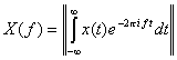
Since frequency is one of the important pieces of information necessary to accurately recognize sound, it is necessary to have a transformation that allows one to break a signal into its frequency components. The most common way to do this is the Fourier transform. The Fourier transform of a signal is the representation of the frequency and amplitude[G1] of that signal. The Fourier transform of a signal can obtained mathematically by the equation 2-1, where i is the imaginary number and the || || represents magnitude.
 (eq.
2-1)
(eq.
2-1)
The Fourier transform of the signal in figure 2-1 would then be given as figure 2-2.
Figure 2-1: x(t)
= cos(2pt) + cos(10pt) + cos(20pt)
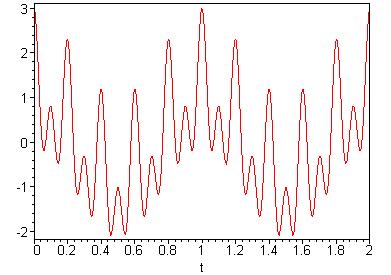
Figure 2-2:
Fourier Transform, X(f), of x(t)
At first glance this seems to be the perfect solution to finding a relation between frequency, time, and amplitude. However, the Fourier transform is missing one the three elements that were necessary to accurately recognize a signal. The Fourier transform gives no respect to where in time each frequency exists. It assumes that each frequency exists over all time. In the previous example that was the case. However, if we look at a signal in which this is not the case the problem will become apparent. Take for example the signal given in figure 2-3 and its Fourier transform in figure 2-4.
Figure 2-3: cos(2pt),
for t = [0,2)
cos(10pt), for t = [2,4)
cos(20pt), for t = [4,6)
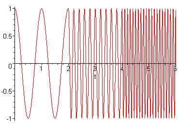
Figure 2-4: Fourier
Transform, X(f), of x(t)
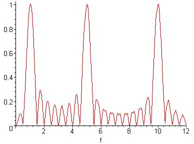
Barring the difference in amplitude and the ‘noise’, the Fourier transforms of the two signals look identical. The signals on the other hand, are very different. It is obvious then how the Fourier transform ignores the location of each frequency. The difference in amplitude at each frequency comes from the fact that the frequencies do not exist over all time. While this fact may help a little, we still would not know where those frequencies do exist. The noise in the Fourier transform is a result of the sudden changes in the time signal. Since the differential of the signal is not continuous, we see these phantom frequencies. However, they are relatively low in amplitude, and can thus be ignored.
Because of this little anomaly with the Fourier transform, it can only be used on signals whose frequency components exist at all times. Such signals are said to be stationary. While this may be great for the mathematical world, the real world is different. Common, everyday signals, such as the signals from speech, are rarely stationary. They will almost always have frequency components that exist for only a short period of time. Therefore, the Fourier transform is rendered an invalid when faced with the task of speech recognition.
2.2 The Short Term Fourier Transform:
The problem with the Fourier Transform is that it looks at too large of an interval. Practical signals are never stationary over their whole domain. However, it is safe to assume that every signal is stationary on some interval. The method would be to break a signal into short intervals of time, and take the Fourier transform over those intervals. This would then give the frequencies that a signal contains, and the location in time of those frequencies.
Take the signal in figure 2-3 as an example. The signal would be divided into windows of length 2 seconds. The first two seconds would then contain a frequency of 1Hz, the second interval would contain a frequency of 5Hz, and the third interval would have a frequency of 10Hz.
Figure 2-4: Short Term
Fourier Transform
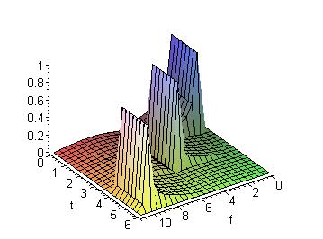
Dividing the signal in figure 2-3 into intervals of the same length would result in each interval containing 1, 5, and 10Hz frequencies. Thus the two signals would be obviously different and very distinguishable.
The Short Term Fourier Transform nicely fixes the problem of knowing when the frequencies occur, but it introduces a new problem. How do you choose a good window? Or more importantly, does a good window exist for speech recognition? Since the human ear is the model for our speech recognition, its limitations should be used as limits for the window size.
The human ear can hear a minimum pitch of 20Hz, and a maximum of 20kHz. Since it would be necessary to have at least 1 period of the lowest frequency in each window, the theoretical minimum window size that can be used is 50ms (the period of 20Hz). However, taking only one period will not give a very good idea of what the frequency is. There could easily exist more nearby frequencies in the given signal. For example, take 1 period of the 20Hz signal in figure 2-5. The Fourier Transform of that signal does not show a precise frequency of 20Hz, it shows a very wide band of frequencies as shown in figure 2-6.
Figure 2-5: 20Hz signal
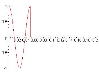
Figure 2-6: The Fourier
Transform
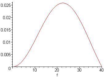
Since there is such a wide bandwidth on the Fourier transform of a single period signal, we can say that the frequency resolution is poor. However, if the time scale is increased by too much, we would have poor time resolution. In fact, in order to get a frequency resolution of about 1Hz, it would be necessary to take 20 periods. This would bring the theoretical minimum window size up from 50ms to 1 second. Considering the fact that people often fit more than one word into a single second, this does not seem a reasonable window. If the window size was to be 1 second then the Short Term Fourier Transform is no better than the Fourier Transform.
3.0 The Wavelet Solution
The Fourier Transform has its difficulties in accurately recognizing voice data, and the Short Term Fourier Transform has problems as well. However, each methodology is very good with a different aspect of the problem. The Fourier Transform resulted in excellent frequency resolution, while the Short Term Fourier Transform provided good time resolution. The obvious solution would be to take the best of both worlds.
In most practical signals, low frequencies are stationary over the length of the signal. High frequencies however, tend to come and go over short intervals of time. Therefore, low frequencies should be analyzed over a longer time interval, and higher frequencies should be checked over a short interval. The result is a multi-resolution analysis, which is essentially the wavelet solution.
A wavelet is, obviously, a small wave, which means that it is defined over a limited period of time. This is commonly referred to as compact support. Thus, the signal is multiplied by a wavelet that has compact support over a defined interval. In the case of the Fourier Transform, the interval is the whole length of the signal. For the Short Term Fourier Transform, the interval can be defined but it remains the same. In the wavelet analysis, the size of this window will change for each frequency. The wavelet signal itself will be the same as is used for the Fourier Transform and the Short Term Fourier Transform.
3.1 High and Low Pass Filters
In order to perform the wavelet analysis it will be necessary to look at only a range of frequencies at a time. Since we want to look at the whole signal when looking for low frequencies, we will want to look at the signal when it only contains low frequencies. In other words, we want to take the high frequencies out. Similarly, when looking for high frequencies we would like to look at a signal that only contains the high frequencies. The reason for taking out the frequencies that we don’t want is so that the transform does not look at, and perhaps get confused by or confuse us with the other frequencies.
The process of taking out unwanted frequencies is known as filtering. After passing a signal through a high pass filter, the signal will only contain frequencies that are above a certain point. All the low frequencies will no longer exist. A low pass filter works the same way, but results in a signal that only contains low frequencies.
For the purposes of the wavelet transform it will be necessary to pass the signal through a series of filters. Take a typical voice signal as an example. The frequencies in this signal will range from 20Hz to 20000Hz. For ease of use, and since 20 is much smaller the 20000, take the range as being 0Hz to 20000Hz. Passing this signal through a low pass filter and then a high pass filter will result in two signals. One signal will contain frequencies ranging from 0Hz to 10000Hz, and the other will have frequencies from 10000Hz to 20000Hz. Passing each of these signals through a high and low pass filter will yield four signals. Each of these signals will contain a range of frequencies; 0Hz to 5000Hz, 5000Hz to 10000Hz, 10000Hz to 15000Hz, and 15000Hz to 20000Hz. Continuing in this manner, you can eventually end up with a number of signals each containing a certain range of frequencies.
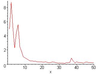
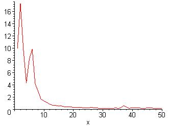
Take the signal in figure 3-1 as an example. This signal is discrete, so the Discrete Fourier Transform, shown in equation 3-1, is used to produce figure 3-2. The Discrete Fourier Transform is symmetric, so the first half of the data is really all that is interesting and so that is all that is shown. Ignore the x-axis and observe the location of the spikes. There are two spikes in the low frequency range, and one spike in the high frequency range.
![]() (eq.
3-1)
(eq.
3-1)
Figure 3-1: Discrete Signal
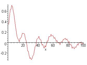
Figure 3-2: Discrete Fourier
Transform
After passing the signal through a low pass filter, seen in equation 3-2, the signal, as shown in figure 3-3, looks like it has lost its high frequencies. The Discrete Fourier Transform of this signal, shown in figure 3-4, verifies that the high frequencies are indeed attenuated.
![]() (eq.
3-2)
(eq.
3-2)
Figure 3-3: Filtered Discrete Signal
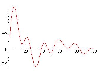
Figure 3-4: Discrete Fourier
Transform
Another method of doing this that would result in the same thing is to pass the original signal through a band pass filter. This filter will take out any frequencies outside the ones contained in a specified range. This method is a lot more straightforward than the one previously mentioned. However, it is more difficult to set up a formula for a band pass filter, so the high and low pass filtering method is generally used.
3.2 Nyquists Criterion
Now that we have the range of frequencies figured out, it will be necessary to find the window of the signal that must be analyzed for each frequency band. Since all the frequency bands are of equal length, the time windows must be of a variety of lengths. This is necessary in order to get the maximum time resolution on each frequency band.
In general, people would not find it obnoxious to speak at a rate of 2 words per second. This would give 1 word every 0.5 seconds. In 0.5 seconds, the lowest frequency that should be analyzed, at 20Hz, will have 10 periods. This will result in a reasonable frequency resolution, as discovered previously.
This will give a starting point from which to calculate the time windows for each of the frequency bands. Nyquists Criterion will provide the relationship between window width and bandwidth. Nyquists Criterion gives the relationship between sampling frequency, N, and desired frequency, f. It is given as:
![]() (eq.
3-3)
(eq.
3-3)
However, the sampling frequency is the inverse of the sampling period, t. This sampling period is the same as the time window that we are looking for. Therefore, equation 3-3 can be written as:
![]() (eq.
3-4)
(eq.
3-4)
Since we have a value for t1, 0.5 seconds, we have a starting point. The frequency values would be determined by the specified bandwidth from the high and low pass filter routine described above. As an example, take the bandwidth as 200Hz, which would result in 100 frequency bands over the signal. The first desired frequency, f1, would then be 200Hz, and the second desired frequency, f2, would be 400Hz. Applying equation 3-4 will result in the value for the second time window, t2. To find the next value for the time window, start with the values for f2 and t2, set f3 to 600Hz (f2 + 200Hz), and apply equation 3-4. Several of these computations are shown in Table 3-1.
Table 3-1: Frequency Bandwidth, and
Time Windows
|
n |
fn
(Hz) |
tn
(s) |
|
1 |
200 |
½ |
|
2 |
400 |
¼ |
|
3 |
600 |
|
|
4 |
800 |
⅛ |
3.3 The Wavelet Coefficients
Now we have all the elements necessary to create the wavelet. The bands of frequency correlate to what is commonly called ‘scale’, and the time windows correlate to time shifting, with Nyquists criterion supplying the compression or dilation. Plotting the frequency bands against the time bands results in figure 3-5. This is strikingly similar to the scale vs. time plot of the Haar wavelets.
Figure 3-5: Frequency Bands vs. Time
Windows
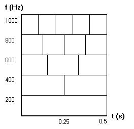
Each wavelet coefficient corresponds to a band of frequencies and a specific window of time. In other words, each box in the Frequency Band vs. Time Window plot will contain a value, the wavelet coefficient for that area in frequency and time. The value of the wavelet coefficient is the maximum amplitude of the harmonic contained in that frequency band. So, if the coefficient for 200Hz to 400Hz in the time range from 0 seconds to 2.5 seconds was 10, we would know that the signal under analysis contained a 200Hz to 400Hz harmonic with an amplitude of 10 between 0 seconds and 0.25 seconds. Similarly, if the coefficient for 600Hz to 800Hz in the time range from 0.325 seconds to 0.5 seconds was 0.1, we would know that the signal contained no 600Hz to 800Hz harmonics from 0.325 seconds to 0.5 seconds.
4.0 Conclusion
The most basic realization in the analysis of voice data for the purpose of recognition is the need for frequency analysis. The best choice for the implementation of frequency analysis has long been the Fourier Transform. The Fourier Transform therefore is a necessary step in voice recognition. However, it has a weakness with voice data because, like most real data, contains frequencies that do not span the length of the signal.
So the second step had to be taken. The Short Term Fourier Transform was brought up because of the need to analyze sections of data. Thus time resolution was introduced. But alas, the Short Term Fourier Transform has weaknesses in analyzing voice data as well. It cannot give a good overall analysis of the signal, so low frequencies, which do exist over much of the signal, are left out of the picture.
All this leads to the final step. The wavelet transform is a mix of the Fourier Transform, and the Short Term Fourier Transform. The wavelet transform utilizes the Fourier Transform to look at the whole signal for low frequencies, and the Short Term Fourier Transform to analyze different sections of the signal, looking for different ranges in frequency. All this adds up to a complete and accurate tool to implement voice recognition.
Appendix A - Maple Code
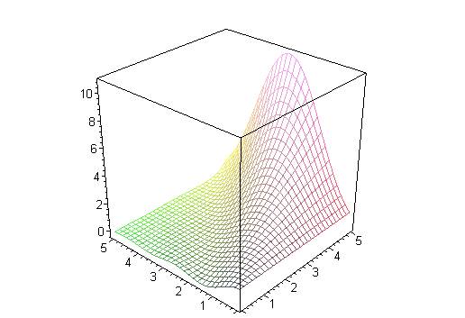
The Cover Sheet Graphic
> restart; with(plots):
> plot3d(binomial,0..5,0..5,grid=[30,30], style=wireframe, axes=boxed);
The Fourier Transform
> restart;
stationary wave
> x := t -> cos(2*Pi*1*t)+cos(2*Pi*5*t)+cos(2*Pi*10*t);
> plot(x(t), t=0..2);
> X := f -> abs(int(x(t)*exp(-2*Pi*I*f*t), t=-10..10));
> plot(X(f), f=0..12);
non-stationary wave
> restart;
> x := t -> piecewise(t<0, 0, 0 <= t and t < 2, cos(2*Pi*1*t), 2 <= t and t < 4, cos(2*Pi*5*t), 4 <= t and t < 8, cos(2*Pi*10*t), 8 <= t, 0);
> plot(x(t), t=0..8);
> X := f -> abs(int(x(t)*exp(-2*Pi*I*f*t), t=-10..10));
> plot(X(f), f=0..12);
The Short Term Fourier Transform
> restart;
> with(plots):
> x1 := t -> piecewise(t<0, 0, 0 <= t and t < 2, cos(2*Pi*1*t), 2 <= t, 0);
> x2 := t -> piecewise(t<2, 0, 2 <= t and t < 4, cos(2*Pi*5*t), 4 <= t, 0);
> x3 := t -> piecewise(t<4, 0, 4 <= t and t < 6, cos(2*Pi*10*t), 6 <= t, 0);
>
> X1 := f -> abs(int(x1(t)*exp(-2*Pi*I*f*t), t=-10..10));
> X2 := f -> abs(int(x2(t)*exp(-2*Pi*I*f*t), t=-10..10));
> X3 := f -> abs(int(x3(t)*exp(-2*Pi*I*f*t), t=-10..10));
>
> h1 := t -> piecewise(t<0, 0, 0 <= t and t < 2, 1, 2 <= t, 0);
> h2 := t -> piecewise(t<2, 0, 2 <= t and t < 4, 1, 4 <= t, 0);
> h3 := t -> piecewise(t<4, 0, 4 <= t and t < 6, 1, 6 <= t, 0);
>
> plot([X1(f), X2(f), X3(f)], f=0..12);
> plot3d(X1(f)*h1(t)+X2(f)*h2(t)+X3(f)*h3(t), f=0..11, t=0..6);
Why it won't work
> restart;
> x := t -> piecewise(t<0, 0, 0<=0.05 and t<0.05, cos(2*Pi*20*t), 0.05<=t, 0);
> plot(x(t), t=0..0.2);
> X := f -> abs(int(x(t)*exp(-2*Pi*I*f*t), t=-1000..1000));
> plot(X(f), f=0..40);
The Low Pass Filter
> restart;
The Original signal
> fname := `N:\\wavelets project\\traffic_traffic.txt`;
> num_points := 100:
> for i from 1 to num_points do XP[i]:=fscanf(fname,`%f`)[1]: od: fclose(fname): evalm(XP):
> X := [[ n, XP[n]] $n=1..num_points]:
> plot(X, x=0..num_points, style = line);
> for k from 1 to num_points do:
> dft[k] := evalf(abs(sum(exp(-I*2*Pi*k*(n-1)/num_points)*XP[n], n=1..num_points))): od:
> DFT := [[ n, dft[n]] $n=1..num_points]:
> plot(DFT, x = 0..num_points/2, style = line);
The Filtered signal
> lpf[1] := XP[1]:
> for k from 1 to num_points do:
> lpf[k+1] := XP[k+1] + 0.5*lpf[k]: od:
> LPF := [[ n, lpf[n]] $n=1..num_points]:
> plot(LPF, x=0..num_points, style = line);
> for k from 1 to num_points do:
> dft[k] := evalf(abs(sum(exp(-I*2*Pi*k*(n-1)/num_points)*lpf[n], n=1..num_points))): od:
> DFT := [[ n, dft[n]] $n=1..num_points]:
> plot(DFT, x = 0..num_points/2, style = line);