An Example Using Fourier Analysis
The following example creates a Fourier Space F3
and determines the projection of a function onto this space. This example was created using Maple 7. In order to conserve space, most of the
Maple code is left out; however, you should still be able to follow along with
the example. [G1]
We can define F3 as the following “Fourier Space” (a Fourier Space is a vector space consisting of sines and cosines):
F3 = {1, cos t, sin t, cos 2t, sin 2t, cos 3t, sin 3t}.
This will be the base for our example. Since this is an orthogonal base (meaning that the inner product of each of its components equals zero), we will use the Orthogonal Decomposition Theorem to help us. Given the following function:
![]()
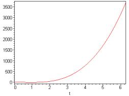
We can determine its projection onto F3. By determining this projection, what we are actually doing is creating a function made up of sines and cosines that can represent our original function h(t). Notice the graph of our original function below.
> plot(h(t),t=0..2*Pi,axes=boxed);
Next, in order to use the Orthogonal Decomposition Theorem, we need to define the inner product (ip) as the integral of the product of two functions from 0 to 2p. Notice below.
Now, we use the Orthogonal Decomposition Theorem to define a new function f using our function h(t) and the Fourier Space F3.
![]()
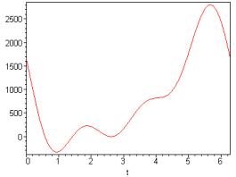
Each of the terms in the function f above creates a coefficient in which the sines and cosines are multiplied by. That is how Fourier was able to change the amplitude (height of the waves) and shift them along the horizontal axis (change the phase). Now, by plotting this new function f(t) in F3(shown below), we will see an oscillating function made up of sines and cosines.
> plot(f(t), t=0..2*Pi, axes=boxed);
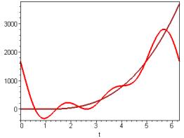
In order to realize the difference between our original function h(t) and our new function f(t), the graph shown on the next page will give a good comparison of the two functions graphed on the same axes (f(t) is in red and h(t) is in brown).
> plot({f(t),h(t)}, t=0..2*Pi, axes=boxed, color=[red,brown],thickness=3);
Lastly, you can also see a big difference in our
projection of h(t) onto F3 by looking at the equations of the two
functions. Below is the equation of our
original h(t).
![]()
Here’s the equation of our projection of h(t) onto F3.
![]()