> restart:

> with(plots):with(linalg):

Warning, the name changecoords has been redefined

Warning, the protected names norm and trace have been redefined and unprotected

> f:=z->1/(2*z^2+3);

Create the Taylor polynomials of degrees Nmin.. Nmax

at z=a for the function f(z):

> a:=0;Nmin:=1; Nmax:=160;

> P:=seq(unapply(convert(taylor(f(z),z=a,n+1),polynom),z),n=Nmin..Nmax):

> P[2](z);P[4](z);P[10](z);

Note how P[n](0)=1/3 for all n, so we know that the Taylor polynomials converge at z0=0. Also, the polynomials

contain only even powers of z. Hence P[n](z)=P[n](-z).

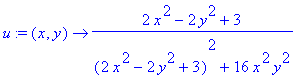
> u:=unapply(evalc(Re(f(x+I*y))),(x,y));

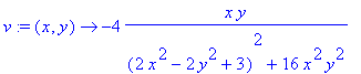
> v:=unapply(evalc(Im(f(x+I*y))),(x,y));

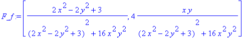
> F_f:=[u(x,y),-v(x,y)];

We want to determine if the Taylor polynomials converge to f(z) at z=z0=x0+i*y0. Thus we'll choose a viewing window centered at z0.

> x0:=.5;y0:=1.1;

> modulus_of_z0:=evalf(sqrt(x0^2+y0^2));

Now choose the size of the viewing window.

> window_size:=.01;

> xmin:=x0-window_size;xmax:=x0+window_size; ymin:=y0-window_size; ymax:=y0+window_size;gridnumber:=5;

> f_field_plot:=fieldplot(F_f,x=xmin..xmax,y=ymin..ymax,arrows=thick,color=red,grid=[gridnumber,gridnumber]):

Here is the Polya field of the function f in a small window centered at z0.

> display(f_field_plot);

> todisplay:=[]:

> for k from Nmin to Nmax do u[k]:=unapply(evalc(Re(P[k](x+I*y))),(x,y)): v[k]:=unapply(evalc(Im(P[k](x+I*y))),(x,y)):F_P[k]:=[u[k](x,y),-v[k](x,y)]: temp_plot:=fieldplot(F_P[k],x=xmin..xmax,y=ymin..ymax,arrows=thick,color=blue,grid=[gridnumber,gridnumber]): new_display:=display([f_field_plot,temp_plot]):todisplay:=[op(todisplay),new_display]: od:

Here is an animation showing various Polya fields. Frame #n of the animation superimposes the

Polya field of f (in red) with the Polya field of the Taylor polynomial of degree n corresponding to f

centered at z=a (in blue). Note what happens as one plots the Taylor polynomial Polya fields of

progressively larger degrees.

Do the Taylor polynomials converge at z=z0?

(You may wish to use the << box in the animate console to decrease the frame rate to 1 frame per second,

or you may wish to use the ->| button to advance one frame at a time.)

> display(todisplay,insequence=true);